This week someone at work asked why GPU acceleration doesn’t exist in commercial powerflow programs. I had a similar question many years ago and wrote a Newton Raphson solver in R that uses the gpuR library. The library hasn’t been updated in 7 years now, is Unix only, requires AMD/nVidia drivers/SDKs, and requires an old version of R like 3.6.3.
The point of this is more of a demonstration though - you can write a GPU accelerated solver relatively easily but GPU support requires libraries and drivers that change often (my attempt is a good case study). Most of the steps like building and ordering the matrix are still CPU tasks as well. Getting a Newton solver is also probably the easiest part. The voltage regulation (LTCs, generator excitation systems, etc.), transient stability, FACTS devices, and more supported and working is another beast entirely. Those algorithms are definitely the secret sauce and tend to be more CPU optimized anyway.
# powerflow convergence tolerance and max iterations
tolerance <- 0.01
max_iterations <- 10

# filename of the basecase
filename <- file.choose()

# read case metadata
metadata <- unlist(strsplit(readLines(file(filename,'r'),1),","))
savcase <- data.frame(nbus=NA,nline=NA,ntran=NA,nbranch=NA)
savcase[,c('nbus','nline','ntran','nbranch')] <- as.numeric(c(metadata[c(4,5,6)],sum(as.numeric(metadata[c(5,6)]))))

# read the bus and branch tables from the case
bus <- read.csv(file=filename, header=FALSE, skip=1, check.names=TRUE, nrows=savcase$nbus)
branch <- read.csv(file=filename, header=FALSE, skip=(savcase$nbus+1), check.names=TRUE, nrows=(savcase$nline+savcase$ntran))[c(-9,-10,-11)]
names(bus) <- c('type','bus','class','v','d','pgen','qgen','pload','qload','kv','xprime')
names(branch) <- c('type','from','to','r','x','b','c','tap')

# Create the PQ and dV vectors
dV <- matrix(c(bus$d[-1],bus$v[-1]),2*(savcase$nbus-1),1)
PQ <- matrix(c(bus$pgen[-1]-bus$pload[-1],bus$qgen[-1]-bus$qload[-1]),2*(savcase$nbus-1),1)

# create Ybus matrix
Ybus <- matrix(0,savcase$nbus,savcase$nbus)
for(i in seq(savcase$nbranch)){
    from <- branch$from[i]
    to <- branch$to[i]
    Ybus[from,from] <- Ybus[from,from] + 1/complex(real=branch$r[i], imaginary=branch$x[i]) + complex(real=0,imaginary=branch$b[i])/2
    Ybus[to,to] <- Ybus[to,to] + 1/complex(real=branch$r[i], imaginary=branch$x[i]) + complex(real=0,imaginary=branch$b[i])/2
    Ybus[from,to] <- Ybus[from,to] - 1/complex(real=branch$r[i], imaginary=branch$x[i])
    Ybus[to,from] <- Ybus[to,from] - 1/complex(real=branch$r[i], imaginary=branch$x[i])
}
print('--------------------------------------------------')
print('Ybus')
print('--------------------------------------------------')
format(Ybus, digits=2)

# Compute magnitude and angle of Ybus
magY <- Mod(Ybus)
angY <- Arg(Ybus)

# count the number of gen buses
ngenbus <- sum(bus$class == 2)

# Calculate the order of the Jacobian matrix
Jorder <- 2*(savcase$nbus-1)

# iterate Newton Raphson's method
mismatch <- 1
iteration <- 0
while(mismatch > tolerance){
    # create Jacobian matrix
    J <- matrix(0,Jorder,Jorder)
    for(k in seq(2, savcase$nbus, 1)){
        for(n in seq(2, savcase$nbus, 1)){
            if(k==n) {
                J[k-1,k-1] <- (-1)*bus$v[k]*sum(magY[-k,n]*bus$v[-k]*sin(bus$d[k]-bus$d[n]-angY[-k,n]))
                J[k-1,k+savcase$nbus-2] <- bus$v[k]*magY[k,k]*cos(angY[k,k])+sum(magY[k,]*bus$v[]*cos(bus$d[k]-bus$d[]-angY[k,]))
                J[k+savcase$nbus-2,k-1] <- bus$v[k]*sum(magY[-k,n]*bus$v[-k]*cos(bus$d[k]-bus$d[-k]-angY[-k,n]))
                J[k+savcase$nbus-2,k+savcase$nbus-2] <- (-1)*bus$v[k]*magY[k,k]*sin(angY[k,k])+sum(magY[k,]*bus$v[]*sin(bus$d[k]-bus$d[]-angY[k,]))
            }
            if(k!=n) {
                J[k-1,n-1] <- bus$v[k]*magY[k,n]*bus$v[n]*sin(bus$d[k]-bus$d[n]-angY[k,n])
                J[k-1,n+savcase$nbus-2] <- bus$v[k]*magY[k,n]*cos(bus$d[k]-bus$d[n]-angY[k,n])
                J[k+savcase$nbus-2,n-1] <- (-1)*bus$v[k]*magY[k,n]*bus$v[n]*cos(bus$d[k]-bus$d[n]-angY[k,n])
                J[k+savcase$nbus-2,n+savcase$nbus-2] <- bus$v[k]*magY[k,n]*sin(bus$d[k]-bus$d[n]-angY[k,n])
            }
        }
    }

    # Drop the row and column of the gen buses in the Jacobian
    J <- J[-(2*which(bus$class %in% 2)), -(2*which(bus$class %in% 2))]

    # Compute the mismatch matrix
    DPQ <- matrix(c(bus$d[-1],bus$v[-1]),2*(savcase$nbus-1),1)
    for(k in seq(2, savcase$nbus, 1)){
        DPQ[k-1] <- PQ[k-1] - bus$v[k]*sum(magY[k,]*bus$v*cos(bus$d[k]-bus$d-angY[k,]))
        DPQ[savcase$nbus+k-2] <- PQ[savcase$nbus+k-2] - bus$v[k]*sum(magY[k,]*bus$v*sin(bus$d[k]-bus$d-angY[k,]))
    }

    # Drop the row of the gen buses in the mismatch matrix
    DPQ <- DPQ[-(2*which(bus$class %in% 2))]
    mismatch <- max(DPQ)

    # import the gpuR library
    #library(gpuR)

    # Copy the Jacobian and mismatch to the GPU
    #gpuJ <- vclMatrix(J, type="float")
    #gpuDPQ <- vclMatrix(matrix(DPQ, ncol=1), type="float")

    # Compute the matrix inverse Jacobian and multiply by DPQ to get the voltage updates
    #gpu_update <- as.matrix(solve(gpuJ) %*% gpuDPQ)

    # Use the Jacobian and the mismatch to calculate the new voltages
    #dV[-(2*which(bus$class %in% 2))] <- dV[-(2*which(bus$class %in% 2))] + gpu_update
    dV[-(2*which(bus$class %in% 2))] <- dV[-(2*which(bus$class %in% 2))] + solve(J) %*% DPQ

    # Update the voltage vectors
    bus$v[-1] <- dV[seq(savcase$nbus,length(dV),1)]
    bus$d[-1] <- dV[seq(1,savcase$nbus-1,1)]

    # increment the iteration counter
    iteration <- iteration + 1

    # Quit program if max iterations is exceeded
    if(iteration > max_iterations){
        print("POWERFLOW DIVERGED!")
        q()
    }

    # print out the result
    cat("Iteration", iteration, "\n")
    print(bus)
}
And here’s a csv formatted case it can solve.
NB,NL,NT,5,3,2,,,,,
3,1,1,1,0,3.948,1.144,0,0,15,0
3,2,3,0.8340619,0,0,0,8,2.8,345,0
3,3,2,1.05,0,5.2,3.376,0.8,0.4,15,0
3,4,3,1.0193533,0,0,0,0,0,345,0
3,5,3,0.9743835,0,0,0,0,0,345,0
1,2,4,0.009,0.1,1.72,12,1,,,
1,2,5,0.0045,0.05,0.88,12,1,,,
1,4,5,0.00225,0.025,0.44,12,1,,,
2,1,5,0.0015,0.02,0,6,1,,,
2,3,4,0.00075,0.01,0,10,1,,,
Finally, here’s an attempt to get it to read a common data format case that programs like PSS/E and PowerWorld can generate but I don’t have that quite working yet.
# filename of the basecase
filename <- "stdin"

# read case metadata
metadata <- unlist(strsplit(readLines(file(filename,'r'),1),","))
savcase <- data.frame(nbus=NA,nline=NA,ntran=NA,nbranch=NA)
savcase[,c('nbus','nline','ntran','nbranch')] <- as.numeric(c(metadata[c(4,5,6)],sum(as.numeric(metadata[c(5,6)]))))

# read the bus and branch tables from the case
bus <- read.csv(file=filename, header=FALSE, skip=1, check.names=TRUE, nrows=savcase$nbus)
print(bus)
branch <- read.csv(file=filename, header=FALSE, skip=(savcase$nbus+1), check.names=TRUE, nrows=(savcase$nline+savcase$ntran))[c(-9,-10,-11)]
names(bus) <- c('type','bus','class','v','d','pgen','qgen','pload','qload','kv','xprime')
names(branch) <- c('type','from','to','r','x','b','c','tap')

# Create the PQ and dV vectors
dV <- matrix(c(bus$d[-1],bus$v[-1]),2*(savcase$nbus-1),1)
PQ <- matrix(c(bus$pgen[-1]-bus$pload[-1],bus$qgen[-1]-bus$qload[-1]),2*(savcase$nbus-1),1)

# create Ybus matrix
Ybus <- matrix(0,savcase$nbus,savcase$nbus)
for(i in seq(savcase$nbranch)){
    from <- branch$from[i]
    to <- branch$to[i]
    Ybus[from,from] <- Ybus[from,from] + 1/complex(real=branch$r[i], imaginary=branch$x[i]) + complex(real=0,imaginary=branch$b[i])/2
    Ybus[to,to] <- Ybus[to,to] + 1/complex(real=branch$r[i], imaginary=branch$x[i]) + complex(real=0,imaginary=branch$b[i])/2
    Ybus[from,to] <- Ybus[from,to] - 1/complex(real=branch$r[i], imaginary=branch$x[i])
    Ybus[to,from] <- Ybus[to,from] - 1/complex(real=branch$r[i], imaginary=branch$x[i])
}

# Compute magnitude and angle of Ybus
magY <- Mod(Ybus)
angY <- Arg(Ybus)

# iterate
for(i in seq(1)){
    # create Jacobian matrix
    J <- matrix(0,2*(savcase$nbus-1),2*(savcase$nbus-1))
    for(k in seq(2, savcase$nbus, 1)){
        for(n in seq(2, savcase$nbus, 1)){
            if(k==n) {
                J[k-1,k-1] <- (-1)*bus$v[k]*sum(magY[-k,n]*bus$v[-k]*sin(bus$d[k]-bus$d[n]-angY[-k,n]))
                J[k-1,k+savcase$nbus-2] <- bus$v[k]*magY[k,k]*cos(angY[k,k])+sum(magY[k,]*bus$v[]*cos(bus$d[k]-bus$d[]-angY[k,]))
                J[k+savcase$nbus-2,k-1] <- bus$v[k]*sum(magY[-k,n]*bus$v[-k]*cos(bus$d[k]-bus$d[-k]-angY[-k,n]))
                J[k+savcase$nbus-2,k+savcase$nbus-2] <- (-1)*bus$v[k]*magY[k,k]*sin(angY[k,k])+sum(magY[k,]*bus$v[]*sin(bus$d[k]-bus$d[]-angY[k,]))
            }
            if(k!=n) {
                J[k-1,n-1] <- bus$v[k]*magY[k,n]*bus$v[n]*sin(bus$d[k]-bus$d[n]-angY[k,n])
                J[k-1,n+savcase$nbus-2] <- bus$v[k]*magY[k,n]*cos(bus$d[k]-bus$d[n]-angY[k,n])
                J[k+savcase$nbus-2,n-1] <- (-1)*bus$v[k]*magY[k,n]*bus$v[n]*cos(bus$d[k]-bus$d[n]-angY[k,n])
                J[k+savcase$nbus-2,n+savcase$nbus-2] <- bus$v[k]*magY[k,n]*sin(bus$d[k]-bus$d[n]-angY[k,n])
            }
        }
    }

    # Compute new dV and PQ matrices
    print(PQ)
    for(k in seq(2, savcase$nbus, 1)){
        PQ[k-1] <- bus$v[k]*sum(magY[k,]*bus$v*cos(bus$d[k]-bus$d-angY[k,]))
        PQ[savcase$nbus+k-2] <- bus$v[k]*sum(magY[k,]*bus$v*sin(bus$d[k]-bus$d-angY[k,]))
    }
    print(PQ)

    dV <- dV + solve(J) %*% PQ

    bus$v[-1] <- dV[seq(savcase$nbus,length(dV),1)]
    bus$d[-1] <- dV[seq(1,savcase$nbus-1,1)]
    #print(bus)
}
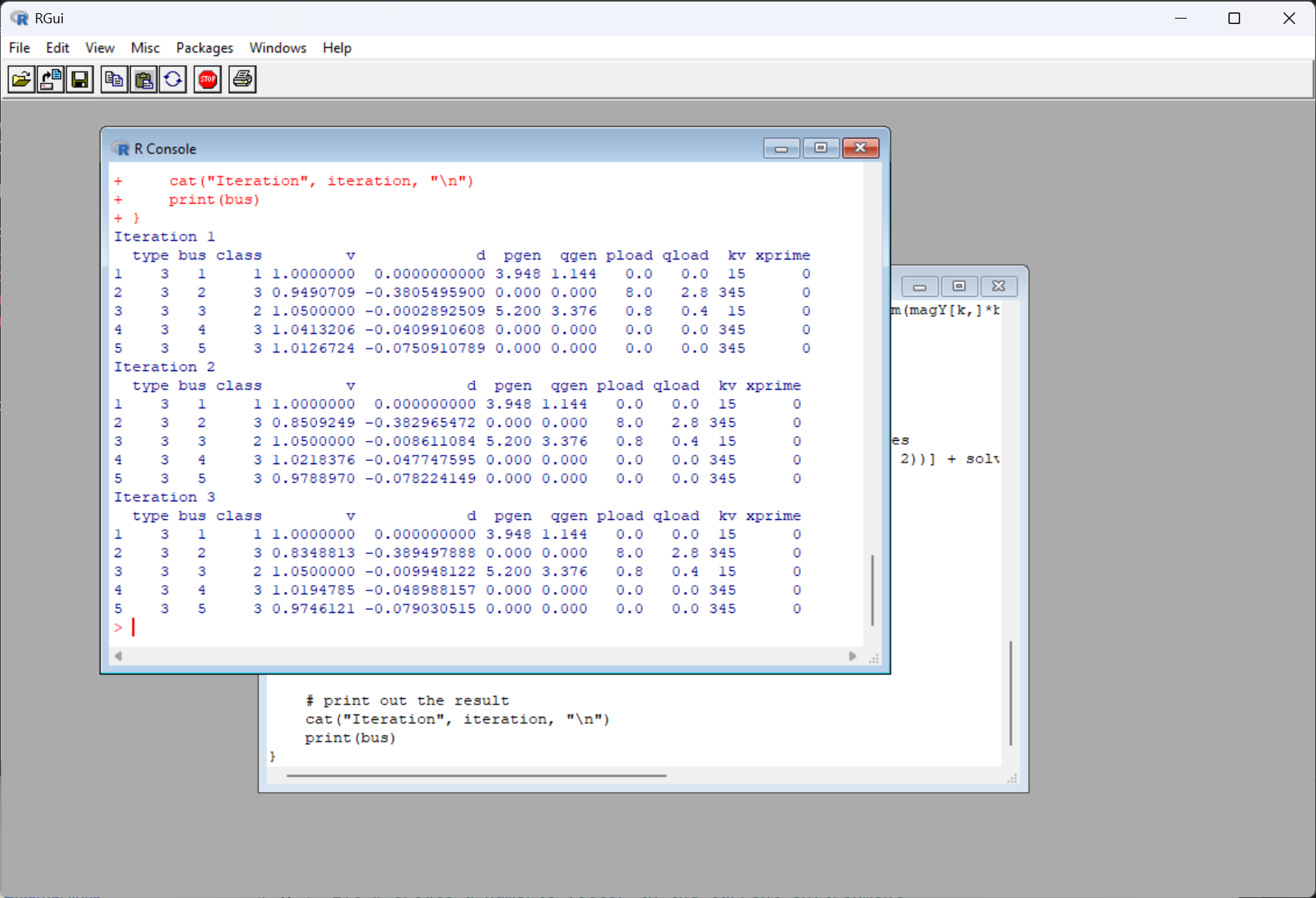
Here’s the result of a solve of that example csv case.